RGB Video Capture(w/o depth) → Surface Reconstruction
(1) Numerical gradients for computing higher-order derivatives as a smoothing operation
(2) coarse-to-fine optimization on the hash grids controlling different levels of details
✨Introduction
배경
Multi-view surface reconstruction Algorithm
- 전통적인 알고리즘 방식
- 반복되는 texture pattern 등 모호한 observation을 다루는 것이 어려움
- noisy/missing surface에 대한 부정확한 reconstruction
Neural Surface reconstruction Methods
- scene을 implicit function으로 나타내기 위해 MLP를 사용
- 최근 multi-resolution hash encoding with lightweight MLP 방식 hybrid를 제안 (Instant NGP) ⇒ Neuralangelo에서 채택
Neuralangelo
- neural SDF representation으로서 Instant-NGP를 채택
- neural surface rendering으로 multi-view image observation optimization
- 논문의 두 가지 주요 findings
(1) “higher order derivative 계산에 있어 numerical gradients를 사용하는 것이 optimization 안정화에 중요한 역할을 한다.”
(2) “progressive optimization schedule이 서로 다른 레벨의 디테일을 가진 structure 복원에 중요한 역할을 한다.”
Contributions
- hash-encoded surface reconstruction의 품질을 향상시키는 두 가지 테크닉을 소개
1. numerical gradients로 higher-order derivatives 계산하기
2. coarse-to-fine optimization with a progressive level of details
⇒ Neural SDF Representation에 multi-resolution hash encoding을 incorporate
✨Approach
목적
multi-view images로부터 scene의 dense structure를 reconstruct하는 것.
요약
1. camera view direction을 따라 3D location을 샘플링
2. multi-resolution hash encoding을 사용하여 position을 encode
3. encoded feature를 input으로 하여 SDF MLP에 집어넣고 SDF-based volume rendering에 사용
※ Pre-preliminaries (3D rendering의 전반적인 이해를 위한 핵심만 요약)
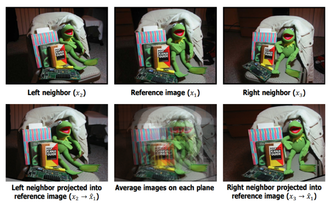
✔ Stereo Matching
- Stereo Matching이란 같은 물체를 서로 다른 각도에서 찍은 이미지들의 픽셀 간 correspondence를 구하는 것을 의미
- 한 pixel을 다른 pixel에 매칭하는 과정에서 depth를 구하는 것이 가능 (차를 타고 이동할 때 가까이 있는 나무는 빠르게 지나가고 멀리있는 풍경은 천천히 움직이는 것처럼 보이는 것과 같은 원리.)
- Matching cost가 가장 적어지는 correspondent point를 찾기 ⇒ 두 point간의 위치 차이(disparity)를 계산하여 disparity map 형성

✔ Multi-view Stereo
- Multi-view Stereo는 서로 다른 각도에서 촬영한 이미지의 개수가 3개 이상이며, 계산 결과가 2D depth map이 아닌 3D shape인 경우를 의미

- 특정 pixel에서의 depth value z를 계속해서 바꿔가며(assumption) reprojection error가 가장 적어지는 z를 찾음
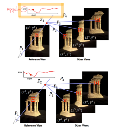
- whole reference view에 대해서 같은 과정을 반복하여 depth map을 구하기
- 이와 같은 매칭을 plane을 sweeping하는 방식으로 진행 (plane-sweep stereo)
✔ SfM
- Multi-view Stereo는 모든 camera가 calibrate되어있다고 가정 (Camera Matrix (R,t)와 K가 모든 view에 대해서 알려져 있다고 가정)
- 실제로는 모든 view가 알려져있지 않음 ⇒ 모든 view를 calibrate하는 것이 불가능.
- 3D structure(X)와 camera location(R,t)에 대해서 모두 assumption을 만들고 reprojection error가 가장 작은 bundle adjustment (X,R,T)를 찾음
😊Preliminaries
각 방식을 채택한 이유
✔ Neural Volume Rendering (NeRF)
특정 pose에 위치해있는 camera와 그 ray direction이 주어졌을 때, ray를 따라서 존재하는 point들의 color radiance를 summision하여 color rendering을 계산

rendered color c는 ray를 따라서 존재하는 point 들의 합임.
- T: How much light is blocked (카메라와 물체 사이를 가로막고 있는 정도)
- α: 물체의 transparency. function of density.
- c: Colors of Point Cloud (RGB)
$$ c \approx \sum_{i=1}^{n}T_{i}\alpha_{i}c_{i} $$
네트워크는 각 location의 color와 density를 배우게 되는 것.
Loss function은 Rendered color image c와 GT image 간의 차이.
$$ L_{RGB} = ||\hat{c} - c||_{1} $$
⇒ 이러한 density formulation를 사용하게 되면 surface가 명확하게 정의되지 않음 → noisy하고 unrealistic한 결과가 나올 수 있음.
✔ Volume Rendering of SDF
가장 널리 사용되는 surface representation
NeRF의 density prediction을 SDF representation으로 변환하는 것을 제안하는 논문이 등장
해당 논문을 차용하여 neural SDF based volume rendering formulation을 사용
✔ Multi Resolution Hash Encoding
multi resolution hash encoding이 neural scene representation에 좋은 scalability를 보여줌
논문에서 high fidelity surface 복원을 위해 representation에 있어 hash encoding을 채택
동작
- multi-resolution 그리드를 사용하는데, 각 그리드 셀의 모서리가 hash entry에 매핑됨
- 각 hash entry는 encoding feature를 저장하고 있음
sparse voxel structure를 사용하지 않는 이유
- Hash Encoding 대신 각 그리드 모서리가 충돌 없이 uniquely하게 정의되는 sparse voxel structure를 사용하는 대안도 존재
- volumetric feature grid는 파라미터를 tractable하게 만들기 위해 hierarchical spatial decomposition을 필요로 함 ⇒ 그렇지 않으면 메모리가 spatial resolution과 함께 cubic하게 증가
- Hash encoding은 spatial hierarchy를 가정하지 않으며, gradient averaging에 기반하여 자동적으로 collision을 해소함.
😊Methods
✔ Numerical Gradient Computation✨✨✨

보통의 hash encoding: Analytical Hash Encoding (첫번째 그림)
SDF의 특징 중 하나는, unit norm으로 ‘미분 가능하다’는 것( SDF의 gradient가 거의 모든 구간에 존재)
SDF에는 보통 eikonal loss가 사용됨
$$ \mathcal{L}{eik} = {1\over N} \sum{i=1}^{N}(||\nabla f(x_{i})||_{2} - 1)^{2} $$
이 때 N은 sample point의 총 개수이며, end-to-end optimization을 위해서 double backward operation이 필요(빨간색 화살표가 두 줄임을 확인. 파란색 동그라미가 grid cell의 범위를 의미)
surface normal 을 계산하는데 있어 analytical gradient를 사용하는 것이 보편적 (position에 대해 hash encoding을 진행). 하지만 trilinear interpolation space에 대해서 연속적이지 못함.
hash encoding의 derivative가 local함 → x_i가 grid cell border를 넘어갈 때, hash entry가 달라지게 됨 → eikonal loss가 locally sampled hash entry에 대해서만 backpropagate하게 됨
연속적인 표면이 필요한(평평한 벽 등) 여러개의 grid cell에 걸쳐 일관적인 surface normal이 필요한 반면 ⇔ analytical gradient는 모든 grid cell이 동시에 샘플링되고 optimize되지 않는 한 local grid cell에만 제한됨, 더군다나 그러한 optimization이 항상 이루어진다는 보장이 없음.
⇒ locality 문제를 겪음 (local has grid에 대해서만 gradient가 최적화되어 non-local smoothness에 부정적인 영향)
numerical gradients 제안 (오른쪽 그림)
surface normal을 numerical gradient로 계산
- hash encoding의 grid size보다 numerical gradient의 step size가 작을 경우: numerical gradient가 analytical gradient와 동일
- 반대 경우: multiple grid cell에 걸친 hash entry가 surface normal computation에 관여. 이 경우 동시에 여러 grid에 걸친 hash entry로 하여금 동시에 optimization되는 것이 가능해짐. (multiple grid cell 파란색 동그라미의 범위가 넓어짐을 확인 + optimization 범위 넓어짐 확인)
+) 거꾸로, 이러한 step size를 surface smoothing 정도를 조정하는 hyperparameter로 해석할 수 있음.(아래 progressive levels of details 참고)
추가 network 없이 locality issue를 해결
numerical surface normal computation을 위해 추가 SDF sample이 필요 → sampled point x 하나당 step size ϵ 안에서 canonical coordinate의 축을 따라 2개의 point를 추가로 sample (그림의 초록색 동그라미)
surface normal의 x-component는 아래 식과 같이 표현됨. (그림의 Numerical Gradient가 어떤 경로로 이어지는지 확인하면 이해 가능)
$$ \nabla_{x}f(x_{i}) = {f(\gamma(x_{i}+\epsilon_{x})) - f(\gamma(x_{i}-\epsilon_{x}))\over 2\epsilon}, \ \ where \ \ \epsilon_{x}=[\epsilon, 0, 0] $$
따라서, numerical surface normal computation에 있어서 총 6개의 (4개의 sampled x 모서리 하나당 additional sample 2개) additional SDF sample이 필요하게 됨.
✔Progressive Levels of Details
1) Step Size
큰 step size ⲉ는surface normal이 큰 스케일에서 일관적이도록 조정함
작은 step size ⲉ는 더 작은 region에 영향을 미치며 smoothing detail을 피함
초기 ⲉ를 coarsest hash grid size로 초기화하고, 최적화 과정에서 exponential하게 그 사이즈를 줄이도록 함
2) Hash Grid Resolution
최적화 과정에서 처음부터 모든 hash grid가 활성화되어있으면 fine hash grid는 coarse optimization 단계에서 “unlearn”하게 되고 다시 smaller ⲉ에 대해서 “relearn”해야 하는 상황 발생
따라서 처음에는 몇 개의 coarse hash grid만 활성화시키고 ⲉ가 작아짐에 따라 점진적으로 fine grid를 활성화시킴 (progressive)
⇒ relearning 현상을 회피가능
✔ Optimization
reconstructed surface의 smoothness를 더 encourage하기 위해서 SDF의 mean curvature를 regularize시킴으로써 prior를 부여함.
$\mathcal{L}{curve} = {1 \over N}\sum^{N}{i=1}|\nabla ^{2}f(x_{i})|$
종합하여 보았을 때, total loss는 아래 loss들의 weighted sum으로 계산됨.
$$ \mathcal{L} = \mathcal{L}{RGB}+w{eik}\mathcal{L}{eik}+w{curv}\mathcal{L}_{curv} $$
MLP, hash encoding을 비롯한 모든 network parameter는 jointly end-to-end 하게 훈련됨 (InstantNGP도 마찬가지.)
😊 Experiments
Dataset, Implementation Details, and Evaluation Criteria.
데이터셋
- 15개의 object-centric scene이 포함된 DTU dataset ⇒ object 하나 당 64개 또는 49개의 이미지로 학습 / GT 는 structured light scanner로 수집
- 큰 scale의 Tanks and Temples dataset ⇒ 263에서 1107이미지 / GT는 LiDAR sensor로 얻음
구현 디테일
- 2^5에서 2^11까지 16개의 level로 hash encoding resolution 구성
- 각 hash entry로 하여금 channel size 8을 가지도록 함.
- dataset마다 다른 scene scale에 따라 optimization 시작 부분의 hash resolution을 달리 함 (4 / 8)
- 5000 iteration마다 새로운 hash resolution을 활성화함 (step size가 grid cell size와 같아질 때)
평가지표
- surface 평가에 대해서는 Chamfer distance와 F1 score 사용
- image synthesis의 질적 평가는 PSNR 사용
DTU

Tanks and Temples Dataset


질적/양적 평가 모두 우수함을 확인